Urban Energy Balance - SUEWS Spatial
Introduction
In this tutorial you will generate input data for the SUEWS model and simulate spatial (and temporal) variations of energy exchanges within a small area on Manhattan (New York City) with regards to a heat wave event.
Tools such as this, once appropriately assessed for an area, can be used for a broad range of applications. For example, for climate services (e.g. http://www.wmo.int/gfcs/ , Baklanov et al. 2018). Running a model can allow analyses, assessments, and long-term projections and scenarios. Most applications require not only meteorological data but also information about the activities that occur in the area of interest (e.g. agriculture, population, road and infrastructure, and socio-economic variables).
This tutorial makes use of local high resolution detailed spatial data. If this kind of data is unavailable, other datasets such as local climate zones (LCZ) from the WUDAPT database could be used. The tutorial Urban Energy Balance - SUEWS and WUDAPT is available if you want to know more about using LCZs in SUEWS. However, it is strongly recommended to go through this tutorial before moving on to the WUDAPT/SUEWS tutorial.
Model output may be needed in many formats depending on a users’ needs. Thus, the format must be useful, while ensuring the science included within the model is appropriate. Fig. 36 shows the overall structure of UMEP, a city based climate service tool (CBCST) used in this tutorial. Within UMEP there are a number of models which can predict and diagnose a range of meteorological processes.
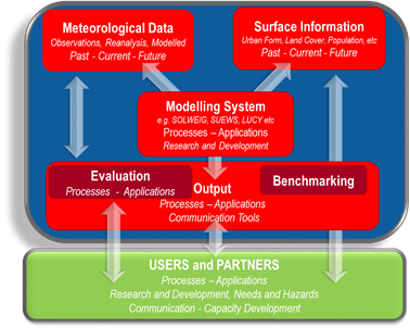
Fig. 36 Overview of the climate service tool UMEP (from Lindberg et al. 2018)
Note
It is recommended that you have a look at the tutorials Urban Energy Balance - SUEWS Introduction and Urban Energy Balance - SUEWS Advanced before you go through this tutorial.
Objectives
To perform and analyse energy exchanges within a small area on Manhattan, NYC.
Overview of Steps
Pre-process the data and create input datasets for the SUEWS model
Run the model
Analyse the results
Perform simple mitigation measures to see how it affects the model results
Initial Steps
UMEP is a Python plugin used in conjunction with QGIS. To install the software and the UMEP plugin see the getting started section in the UMEP manual.
Loading and analyzing the spatial data
All the geodata used in this tutorial is from open access sources, primarily from New York City. Information about the data is found in the table below.
Note
You can download the all the data from here. Unzip and place in a folder that you have read and write access to.
Geodata |
Year |
Source |
Description |
Digital surface model (DSM) |
2013 (Lidar), 2016 (building polygons) |
United States Geological Survey (USGS). New York CMGP Sandy 0.7m NPS Lidar and NYC Open Data Portal: link |
A raster grid including both buildings and ground given in meter above sea level. |
Digital elevation model (DEM) |
2013 |
United States Geological Survey (USGS). New York CMGP Sandy 0.7m NPS Lidar: link |
A raster grid including only ground heights given in meter above sea level. |
Digital canopy model (CDSM) |
2013 (August) |
United States Geological Survey (USGS). New York CMGP Sandy 0.7m NPS Lidar: link |
A vegetation raster grid where vegetation heights is given in meter above ground level. Vegetation lower than 2.5 meter pixels with no vegetation should be zero. |
Land cover (UMEP formatted) |
2010 |
New York City Landcover 2010 (3ft version). University of Vermont Spatial Analysis Laboratory and New York City Urban Field Station: link |
A raster grid including: 1. Paved surfaces, 2. Building surfaces, 3. Evergreen trees and shrubs, 4. Deciduous trees and shrubs, 5. Grass surfaces, 6. Bare soil, 7. Open water |
Population density (residential) |
2010 |
2010 NYC Population by Census Tracts, Department of City Planning (DCP): link |
People per census tract converted to pp/ha. Converted from vector to raster. |
Land use |
2018 |
NYC Department of City Planning, Technical Review Division: link |
Used to redistribute population during daytime (see text). Converted from vector to raster |
Start by loading all the raster datasets into an empty QGIS project.
The order in the Layers Panel determines what layer is visible. You can choose to show a layer (or not) with the tick box. You can modify layers by right-clicking on a layer in the Layers Panel and choose Properties. Note for example that that CDSM (vegetation) is given as height above ground (meter) and that all non-vegetated pixels are set to zero. This makes it hard to get an overview of all 3D objects (buildings and trees). QGIS default styling for a raster is using the 98 percentile of the values. Therefore, not all the range of the data is shown in the layer window to the left.
Right-click on your CDSM layer and go to Properties > Style and choose Singleband pseudocolor with a min value of 0 and max of 35. Choose a colour scheme of your liking.
Go to Transparency and add an additional no data value of 0. Click ok.
Now put your CDSM layer at the top and your DSM layer second in your Layers Panel. Now you can see both buildings and vegetation 3D object in your map canvas.
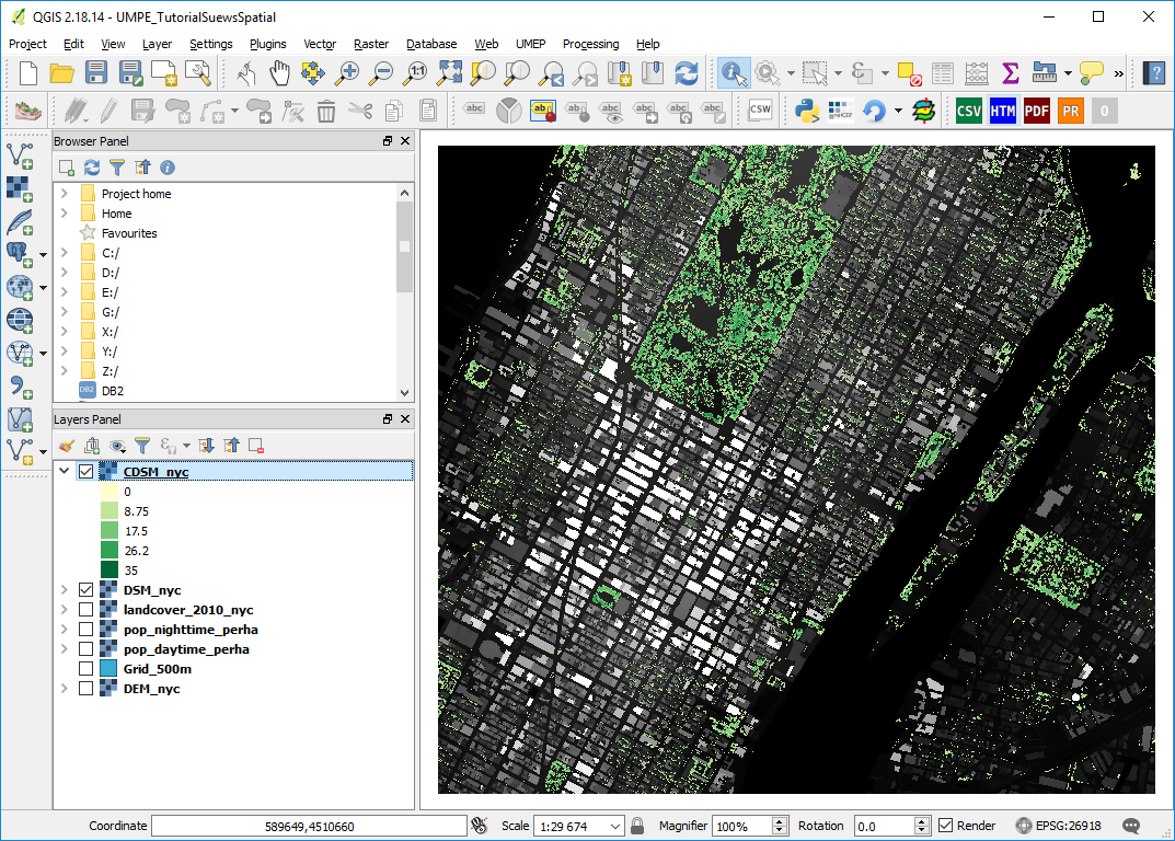
Fig. 37 DSM and CDSM visible at the same time (click for larger image)
The land cover grid comes with a specific QGIS style file.
Right-click on the land cover layer (landcover_2010_nyc) and choose Properties. At the bottom left of the window there is a Style-button. Choose Load Style and open landcoverstyle.qml and click OK.
Make only your land cover class layer visible to examine the spatial variability of the different land cover classes.
The land cover grid has already been classified into the seven different classes used in most UMEP applications (see Land Cover Reclassifier). If you have a land cover dataset that is not UMEP formatted you can use the Land Cover Reclassifier found at UMEP > Pre-processor > Urban Land Cover > Land Cover Reclassifier in the menu-bar to reclassify your data.
Furthermore, a polygon grid (500 m x 500 m) to define the study area and individual grids is included (Grid_500m.shp). Such a grid can be produced directly from the Processing Toolbox in QGIS (Create Grid) or an external grid can be used.
Load the vector layer Grid_500m.shp into your QGIS project.
In the Symbology tab in layer Properties, choose a Simple fill and set Fill style to No Brush, to be able to see the spatial data within each grid.
Also, add the label IDs for the grid to the map canvas in Properties > Labels > Single Labels to make it easier to identify the different grid squares later on in this tutorial.
As you can see, the grid does not cover the whole extent of the raster grids. This is to reduce computation time during the tutorial. One grid cell takes ~20 s to model with SUEWS with meteorological forcing data for a full year.
Meteorological forcing data
Meteorological forcing data is mandatory for most of the models within UMEP. The UMEP specific format is given in Table 5. Some of the variables are optional and if not available or not needed should be set to -999. The columns can not be empty. The needed data for this tutorial is discussed below.
No. |
Header |
Description |
Accepted range |
Comments |
|---|---|---|---|---|
1 |
iy |
Year [YYYY] |
Not applicable |
|
2 |
id |
Day of year [DOY] |
1 to 365 (366 if leap year) |
|
3 |
it |
Hour [H] |
0 to 23 |
|
4 |
imin |
Minute [M] |
0 to 59 |
|
5 |
qn |
Net all-wave radiation [W m-2] |
-200 to 800 |
|
6 |
qh |
Sensible heat flux [W m-2] |
-200 to 750 |
|
7 |
qe |
Latent heat flux [W m-2] |
-100 to 650 |
|
8 |
qs |
Storage heat flux [W m-2] |
-200 to 650 |
|
9 |
qf |
Anthropogenic heat flux [W m-2] |
0 to 1500 |
|
10 |
U |
Wind speed [m s-1] |
0.001 to 60 |
|
11 |
RH |
Relative Humidity [%] |
5 to 100 |
|
12 |
Tair |
Air temperature [°C] |
-30 to 55 |
|
13 |
pres |
Surface barometric pressure [kPa] |
90 to 107 |
|
14 |
rain |
Rainfall [mm] |
0 to 30 |
(per 5 min) this should be scaled based on time step used |
15 |
kdown |
Incoming shortwave radiation [W m-2] |
0 to 1200 |
|
16 |
snow |
Snow [mm] |
0 to 300 |
(per 5 min) this should be scaled based on time step used |
17 |
ldown |
Incoming longwave radiation [W m-2] |
100 to 600 |
|
18 |
fcld |
Cloud fraction [tenths] |
0 to 1 |
|
19 |
wuh |
External water use [m3] |
0 to 10 |
(per 5 min) scale based on time step being used |
20 |
xsmd |
(Observed) soil moisture |
0.01 to 0.5 |
[m3 m-3 or kg kg-1] |
21 |
lai |
(Observed) leaf area index [m2 m-2] |
0 to 15 |
|
22 |
kdiff |
Diffuse shortwave radiation [W m-2] |
0 to 600 |
|
23 |
kdir |
Direct shortwave radiation [W m-2] |
0 to 1200 |
Should be perpendicular to the Sun beam. One way to check this is to compare direct and global radiation and see if kdir is higher than global radiation during clear weather. Then kdir is measured perpendicular to the solar beam. |
24 |
wdir |
Wind direction [°] |
0 to 360 |
The meteorological dataset used in this tutorial (MeteorologicalData_NYC_2010.txt) is from NOAA (most of the meteorological variables) and NREL (solar radiation data). It consists of tab-separated hourly air temperature, relative humidity, incoming shortwave radiation, pressure, precipitation and wind speed for 2010. There are other possibilities within UMEP to acquire meteorological forcing data. The pre-processor plugin WATCH can be used to download the variables needed from the global WATCH forcing datasets (Weedon et al. 2011, 2014).
Open the meteorological dataset (MeteorologicalData_NYC_2010.txt) in a text editor of your choice. As you can see it does not include all the variables shown in Table 5. However, these variables are the mandatory ones that are required to run SUEWS. In order to format (and make a quality check) the data provided into UMEP standard, you will use the MetPreProcessor.
Open MetDataPreprocessor (UMEP> Pre-Processor -> Meteorological Data > Prepare existing data).
Load MeteorologicalData_NYC_2010.txt and make the settings as shown below. Name your new dataset NYC_metdata_UMEPformatted.txt.
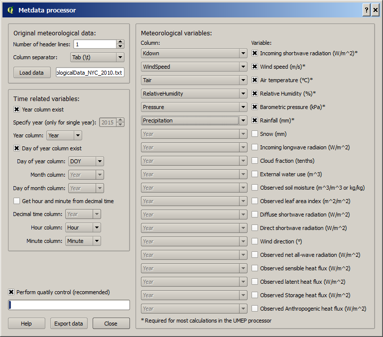
Fig. 38 The settings for formatting met data into UMEP format (click for a larger image)
Close the Metdata preprocessor and open your newly fomatted datset in a text editor of your choice. Now you see that the forcing data is structured into the UMEP pre-defined format.
Close your text file and move on to the next section of this tutorial.
Preparing input data for the SUEWS model
A key capability of UMEP is to facilitate preparation of input data for the various models. SUEWS requires input information to model the urban energy balance. The plugin SUEWS Prepare serves this purpose. This tutorial makes use of high resolution data but WUDAPT datasets, in-conjuction with the LCZ Converter, can be used (UMEP > Pre-Processor > Spatial data > LCZ Converter).
Open SUEWS Prepare (UMEP > Pre-Processor > Urban Energy Balance (SUEWS) > SUEWS prepare).
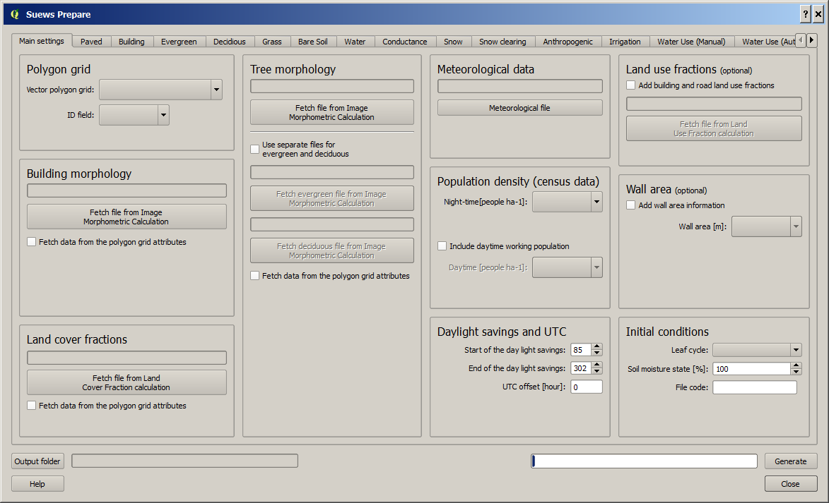
Fig. 39 The dialog for the SUEWS Prepare plugin (click for a larger image).
Here you can see the various settings that can be modified. You will focus on the Main Settings-tab where the mandatory settings are chosen. The other tabs include the settings for e.g. different land cover classes, human activities etc.
There are 10 frames included in the Main Settings tab where 8 need to be filled in for this tutorial:
Polygon grid
Building morphology
Tree morphology
Land cover fractions
Meteorological data
Population density
Daylight savings and UTC
Initial conditions
The two optional frames (Land use fractions and Wall area) should be considered if the ESTM model is used to estimate the storage energy term (Delta QS). In this tutorial we use the OHM modelling scheme so these two tabs can be ignored for now.
Close SUEWS Prepare
Building morphology
First you will calculate roughness parameters based on the building geometry within your grids.
Open UMEP > Pre-Processor > Urban Morphology > Morphometric Calculator (Grid).
Use the settings as in the figure below and press Run.
When calculation ids done, close the plugin.
Note
For mac users, use this workaround: manually create a directory, go into the folder above and type the folder name. It will give a warning “—folder name–” already exists. Do you want to replace it? Click replace.
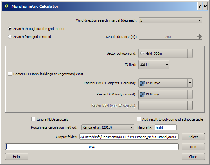
Fig. 40 The settings for calculating building morphology.
This operation should have produced 17 different text files; 16 (anisotrophic) that include morphometric parameters from each 5 degree section for each grid and one file (isotropic) that includes averaged values for each of the 16 grids. You can open build_IMPGrid_isotropic.txt and compare the different values for a park grid (3054) and an urban grid (3242). Header abbreviations are explained here.
Tree morphology
Now you will calculate roughness parameters based on the vegetation (trees and bushes) within your grids. As you noticed there is only one surface dataset for vegetation present (CDSM_nyc) and if you examine your land cover grid (landcover_2010_nyc) you can see that there is only one class of high vegetation (Deciduous trees) present with our model domain. Therefore, you will not separate between evergreen and deciduous vegetation in this tutorial. As shown in Table 4, the tree surface model represents height above ground.
Again, Open UMEP > Pre-Processor > Urban Morphology > Morphometric Calculator (Grid).
Use the settings as in the figure below and press Run.
When calculation is done, close the plugin.
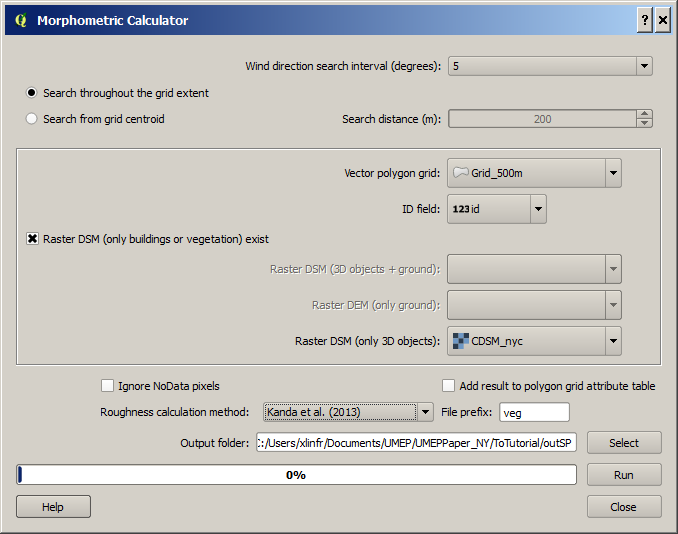
Fig. 41 The settings for calculating vegetation morphology.
Land cover fractions
Moving on to land cover fraction calculations for each grid.
Open UMEP > Pre-Processor > Urban Land Cover > Land Cover Fraction (Grid).
Use the settings as in the figure below and press Run.
When calculation is done, close the plugin.
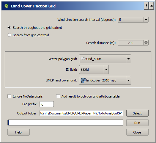
Fig. 42 The settings for calculating land cover fractions
Population density
Population density will be used to estimate the anthropogenic heat release (QF) in SUEWS. There is a possibility to use both night-time and daytime population densities to make the model more dynamic. You have two different raster grids for night-time (pop_nighttime_perha) and daytime (pop_daytime_perha), respectively. This time you will make use of QGIS built-in function to to acquire the population density for each grid.
In the Processing Toolbox, search for Zonal Statistics. Open the tool.
Choose your pop_daytime_perha layer as Raster layer and your Grid_500m as the vector layer. Use a Output column prefix of PPday and chose only to calculate Mean. Click OK.
Run the tool again but this time use the night-time dataset (PPnight).
SUEWS Prepare
Now you are ready to organise all the input data into the SUEWS input format.
Open UMEP > Pre-Processor > SUEWS Prepare
In the Polygon grid frame, choose your polygon grid (Grid_500m) and choose id as your ID field
In the Building morphology frame, fetch the file called build_IMPGrid_isotropic.txt.
In the Land cover fractions frame, fetch the file called lc_LCFG_isotropic.txt.
In the Tree morphology frame, fetch the file called veg_IMPGrid_isotropic.txt.
In the Meteorological data frame, fetch your UMEP formatted met forcing data text file.
In the Population density frame, choose the appropriate attributes created in the previous section for daytime and night-time population density.
In the Daylight savings and UTC frame, set start and end of the daylight saving to 87 and 304, respectively and choose -5 (i.e. the time zone).
In the Initial conditions frame, choose Winter (0%) in the Leaf Cycle, 100% Soil moisture state and nyc as a File code.
In the Anthropogenic tab, change the code to 771. This will make use of settings adjusted for NYC according to Sailor et al. 2015.
Choose an empty directory as your Output folder in the main tab.
Press Generate
When processing is finished, close SUEWS Prepare.
Running the SUEWS model in UMEP
To perform modelling energy fluxes for multiple grids, Urban Energy Balance - SUEWS Advanced can be used.
Open UMEP > Processor > Urban Energy Balance > SUEWS/BLUEWS, Advanced. Here you can change some of the run control settings in SUEWS. SUEWS can also be executed outside of UMEP and QGIS (see SUEWS Manual). This is recommended when modelling long time series (multiple years) of large model domains (many grid points).
Change the OHM option to [1]. This allows the anthropogenic energy to be partitioned also into the storage energy term.
Leave the rest of the combobox settings at the top as default and tick both the Use snow module and the Obtain temporal resolution… boxes.
Set the Temporal resolution of output (minutes) to 60.
Locate the directory where you saved your output from SUEWSPrepare earlier and choose an output folder of your choice.
Also, Tick the box Apply spin-up using…. This will force the model to run twice using the conditions from the first run as initial conditions for the second run.
Click Run. This computation will take a while so be patient.
Analysing model reults
UMEP has a tool for basic analysis of any modelling performed with the SUEWS model. The SUEWSAnalyser tool is available from the post-processing section in UMEP.
Open UMEP > Post-Processor > Urban Energy Balance > SUEWS Analyzer. There are two main sections to this tool. The Plot data-section can be used to do temporal analysis as well as making simple comparisons between two grids or variables. The Spatial data-section can be used to make aggregated maps of the output variables from the SUEWS model. This requires that you have loaded the same polygon grid into your QGIS project that was used when you prepared the input data for SUEWS using SUEWS Prepare earlier in this tutorial.
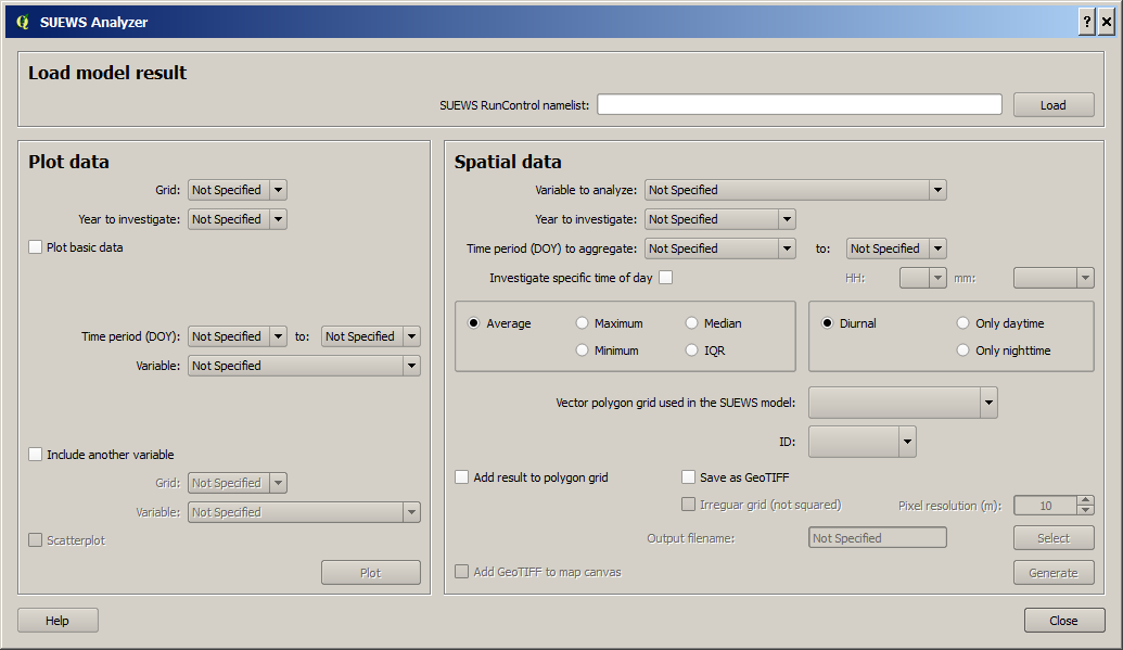
Fig. 43 The dialog for the SUEWS Analyzer tool.
To access the output data from the a model run, the RunControl.nml file for that particular run must be located. If your run has been made through UMEP, this file can be found in your output folder. Otherwise, this file can be located in the same folder from where the model was executed.
In the top panel of SUEWS Analyzer, load the RunControl.nml located in the output folder.
You will start by plotting basic data for grid 3242 which is one of the most dense urban areas in the World.
In the left panel, choose grid 3242 and year 2010. Tick plot basic data and click Plot. This will display some of the most essential variables such as radiation balance, energy budget etc. You can use the tools such as the zoom to examine a shorter time period more in detail.
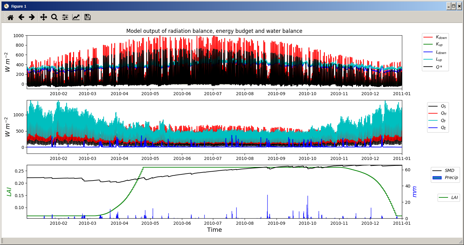
Fig. 44 Basic plot for grid 3242. Click on image for enlargement.
Notice e.g. the high QF values during winter as well as the low QE values throughout the year.
Close the plot and make the same kind of plot for grid 3054 which is a grid mainly within Central Park. Consider the differences between the plot generated for grid 3242. Close the plot when you are done.
From the left panel, it is also possibile to examine two different variables in time, either from the same grid or between two different grid points. It is also possible to examine different parameters through scatterplots.
The right panel in SUEWS Analyzer can be used to perform basic spatial analysis on your model results by producing aggregated maps etc, using different variables and time spans. Sensible heat (QH) is one variable to visualise warm areas as it is a variable that shows the amount of the available energy that will be partitioned into heat.
Make the settings as shown in the figure below but change the location where you will save your data on your own system.
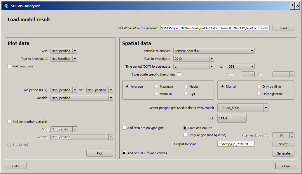
Fig. 45 The dialog for the SUEWS Analyzer tool to produce a mean QH for each grid. Click on image for enlargement.
Note that the warmest areas are located in the most dense urban environments and the coolest are found where either vegetation and/or water bodies are present. During 2010 there was a 3-day heat-wave event in the region around NYC that lasted from 5 to 8 July 2010 (Day of Year: 186-189).
Make a similar average map but this time of 2m air temperature and choose only the heat wave period. Save it as a separate geoTiff.
The influence of mitigation measures on the urban energy balance (optional)
There are different ways of manipulating the data using UMEP, as well as directly changing the input data in SUEWS, to examine the influence of mitigation measures on the urban energy balance (UEB). The most detailed way would be to directly change the surface data by, for example, increasing the number of street trees. This can be done by using the TreeGenerator-plugin in UMEP, for example. This method would require that you go through the workflow of this tutorial again before you do your new model run. Another way is to directly manipulate input data to SUEWS at grid point level. This can done by e.g. changing the land cover fractions in SUEWS_SiteSelect.txt, the file that includes all grid-specific information used in SUEWS.
Make a copy of your whole input folder created from SUEWSPrepare earlier and rename it to e.g. Input_mitigation.
In that folder remove all the files beginning with InitialConditions except the one called InitialConditionsnyc_2010.nml.
Open SUEWS_SiteSelect.txt in Excel (or similar software).
Now increace the fraction of decidious trees (Fr_DecTr) for grid 3242 and 3243 by 0.2. As the total land cover fraction has to be 1 you also need to reduce the paved fraction (Fr_Paved) by the same amount.
Save and close. Remember to keep the format (tab-separated text).
Create an empty folder called Output_mitigation
Open SuewsAdvanced and make the same settings as before but change the input and output folders.
Run the model.
When finished, create a similar average air temperature map for the heat event and compare the two maps. You can create a difference map by using the Raster Calculator in QGIS (Raster>Raster Calculator…).
Tutorial finished.