Solar Energy - Introduction to SEBE

Introduction

Lindberg et al.’s (2015) solar radiation model SEBE (Solar Energy on Building Envelopes) allows estimates of solar irradiance on ground surfaces, building roofs and walls. It uses a shadow casting algorithm with a digital surface model (DSM) and the solar position to generate pixel-level information of shadow or sunlit areas. The shadow casting algorithm (Ratti and Richens 1999) has been developed to incorporate walls (Lindberg et al. 2015). This is of interest for a broad range of applications, for example solar energy potential and thermal comfort.

SEBE is incorporated in UMEP (Urban Multi-scale Environmental Predictor), a plugin for QGIS. As SEBE was initially developed to estimate solar energy potential on building roofs, the Digital Surface Models (DSMs) used need to include roof structures, such as tilted roofs, chimneys etc. Methods to produce accurate ground and building DSMs for SEBE include the use of LiDAR technology and 3D roof structure objects in vector format.

In this exercise you will apply the model in Gothenburg, Sweden and Covent Garden, London to investigate solar energy potential, how it changes between buildings, with seasons, with the effects of vegetation etc.

Initial Practical steps

• If QGIS and UMEP is not on your computer you will need to install it

• Start the QGIS software

• Windows: If not visible on the desktop use the Start button to find the software (i.e. Find QGIS under your applications)

• Select QGIS 3.12 Desktop (or the latest version installed).

When you open it on the top toolbar you will see UMEP.

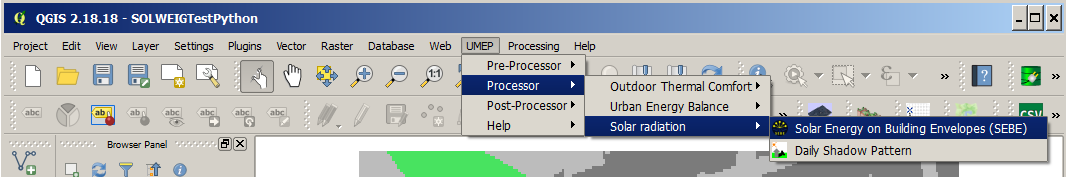
Fig. 5 Location of SEBE in UMEP

• You are recommended to read through the section in the online manual BEFORE using the model, so you are familiar with it’s operation and terminology used.

Data for Tutorial

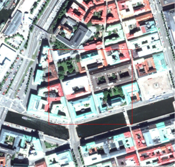
Fig. 6 Central Gothenburg study area (red square). The QuickMapServices-plugin in QGIS was used to generate this snapshot.

Geodata and meteorological data for Gothenburg, Sweden.

• Data is projected in SWEREF99 1200 (EPSG:3007) the national coordinate system of Sweden.

Data requreiments: S: Spatial, M: Meteorological,

Table 2 Input data and parameters found in the Gothenburg dataset

Name	Definition	Type	Description
DSM_KRbig.tif	Ground and building DSM	S	Raster dataset: derived from a 3D vector roof structure dataset and a digital elevation model (DEM)
CDSM_KRbig.asc	Vegetation canopy DSM	S	Raster dataset: derived from a LiDAR dataset
buildings.shp	Building footprint polygon layer	S	Vector dataset
GBG_TMY_1977.txt	Meteorological forcing data	M	Meteorological data, hourly time resolution for 1977 Gothenburg, Sweden

Datasets in Gothenburg, Sweden

Datasets in London Covent Garden

Google map link to Covent Garden

Steps

1. Start with the Gothenbrug data. The data is zipped - unzip the data first.

2. Examine the geodata by adding the layers to your project.

3. Use Layer > Add Layer > Add Raster Layer to open the .tif and .asc raster files and Layer > Add Layer > Add Vector Layer. The Vector layer is a shape file which consists of multiple files. It is the building.shp that should be used to load the vector layer into QGIS.

4. You will need to indicate the coordinate reference system (CRS) for the CDSM_KRbig.asc dataset.

   • Right-click on CDSM_KRbig and go to Layer CRS > Set Layer CRS…. Choose EPSG:3007. You can use the filter to search for the correct CRS.

5. Open the meteorological (GBG_TMY_1977.txt) file in a text editor or in a spreadsheet such as MS excel or LibreOffice (Open office).

   • Data file is formatted for the UMEP plugin (in general) and the SEBE plugin (in particular).

   • First four columns are time related.

   • Columns of interest are kdown (global irradiance on the horizontal plane), kdiff (diffuse irradiance on the horizontal plane) and kdir (beam/direct irradiance on a plane always normal to sun rays).

   • All columns must be present but can be filled with numbers to indicate they are not in use (e.g. -999).

   • The meteorological file should preferably be at least a year long. Multi-year data improves the solar energy estimation.

   • One option is to use a typical meteorological year as you will do in this tutorial

For more details on the meteorological file structure in UMEP, see the meteorological data preprocessor.

Variables included in the meteorological data file:

No. indicates the column of the variable in the file. Use indicates if it is R – required or O- optional (in this application) or N- Not used in this application.

Preparing data for SEBE

Required inputs

SEBE plugin: located at UMEP > Processor > Solar Radiation > Solar Energy on Building Envelopes (SEBE) in the menu bar.

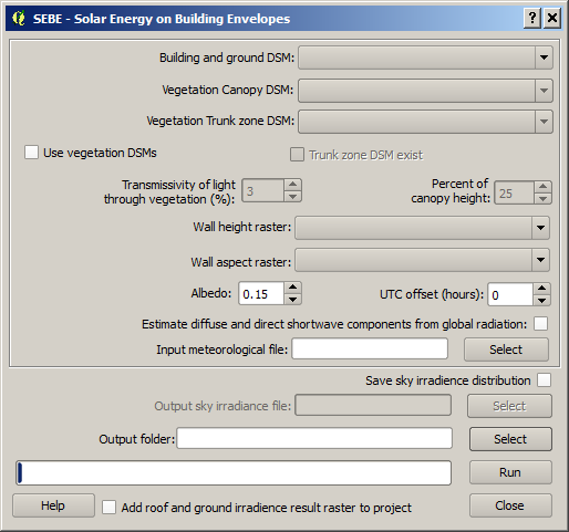
Fig. 7 The interface for SEBE in UMEP

1. Building and ground DSM’s.

   • Critical for the calculations in SEBE is the building and ground DSM.

   • Optionally vegetation (trees and bushes) can be included as they can shadow ground, walls and roofs reducing the potential solar energy production.

   • Two vegetation DSMs are required when the Use vegetation DSMs is ticked:

     • One to describe the top of the vegetation (Vegetation Canopy DSM).

     • One to describe the bottom, underneath the canopies (Vegetation Trunk Zone DSM).

     As Trunk Zone DSMs are very rare, an option to create this from the canopy DSM is available. You can set the amount of light (shortwave radiation) that is transmitted through the vegetation.

2. Two raster datasets, height and wall aspect, are needed to calculate irradiance on building walls.

3. The average albedo (one value is used for all surfaces) can be changed.

4. The UTC offset is needed to accurately estimate the sun position; positive numbers for easterly positions, relative to the prime meridian, and negative for westerly. For example, Gothenburg is located in CET timezone which is UTC +1. The UTC is related to the meteorological forcing data so if ERA5 data is used, UTC should be equal to zero.

5. The meteorological file needs to be specified.

Pre-processing: wall height and aspect

1. Wall data is created with the UMEP plugin - Wall Height and Aspect:

   • The wall height algorithm uses a 3 by 3 pixels kernel minimum filter where the four cardinal points (N, W, S,E) are investigated. The pixels just ‘inside’ the buildings are identified and give values to indicate they are a building edge. The aspect algorithm originates from a linear filtering technique (Goodwin et al. 2009). It identifies the linear features plus (a new addition) the aspect of the identified line. Other more accurate techniques include using a vector building layer and spatially relating this to the wall pixels.

2. Close the SEBE plugin (if open) and open the Wall and Height and Aspect plugin (UMEP > Pre-Processor > Urban Geometry > Wall Height and Aspect).

3. Use your ground and building DSM (in this case DSM_KRbig) as input.

4. Tick the option to Calculate wall aspect.

5. Create a folder in your Documents folder called e.g. SEBETutorial.

6. Name your new raster datasets wallaspect.tif and wallheight.tif, respectively, and save them in your SEBETutorial folder.

7. Tick Add result to project

8. Click Run to create the rasters.

9. Once the window stating that it has run successfully appears, you can close the Wall Height window.

Running the model

Now you have all data ready to run the model.

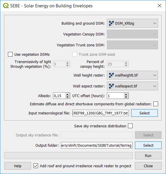
Fig. 8 Example of settings for running SEBE without vegetation.

1. First run the model without including vegetation.

   • Open the SEBE-plugin.

   • Configure the settings according to the figure above.

   • Save your results in a subfolder (NoVeg) of SEBETutorial.

   • The model takes some time to calculate irradiance on all the surfaces.

   • The result added to your map canvas is the horizontal radiation, i.e. irradiance on the ground and roofs.

2. Run the model again but this time also use the vegetation DSM.

   • Save your result in a subfolder called Veg.

Irradiance on building envelopes

Note

Currently, this section works only on a windows computer. 3D Visualisation for Mac and Linux currently not working properly

To determine the irradiance on building walls:

1. Open the SunAnalyser located at UMEP > Post-Processor > Solar Radiation > SEBE (Visualisation).

   • This can be used to visualize the irradiance on both roofs and walls.

2. Choose the input folder where you saved your result for one of the runs.

3. Click Area of Visualisation

4. Click once on the canvas to initiate the visualisation area and then drag to produce an area

5. Click again to finish.

6. Click Visualise. Now you should be able to see the results in 3D.

Use the Profile tool, which is a plugin for QGIS, to see the range of values along a transect.

1. Plugins > Profile tool > Terrain profile. If this is not installed you will need to install it from official QGIS-plugin reporistory (Plugins > Manage and Install Plugins).

   • Draw a line across the screen on the area of interest. Double click and you will see the profile drawn. Make certain you use the correct layer (see Tips).

Solar Energy Potential

In order to obtain the solar energy potential for a specific building:

1. The actual area of the roof needs to be considered.

2. Determine the area of each pixel (A_P): e.g. 1 m²

3. As some roofs are tilting the area may be larger for some pixels. The actual area (A_A) can be computed from:

   A_A = A_P / cos(S_i)

   where the slope (S_i) of the raster pixel should be in radians (1 deg = pi/180 rad).

To create a slope raster:

1. Raster > Analysis > Slope.

2. Use the DSM for the elevation layer.

3. Create the slope z factor =1 - area

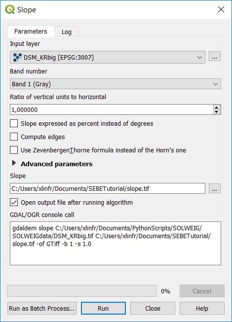
Fig. 9 The Slope tool in QGIS3

1. Now determine the area after you have removed the wall area ( assumed to have slope greater than 65) from the buildings

2. Open the raster calculator: Raster > Raster Calculator.

3. Enter the equation indicated in the figure below.

   

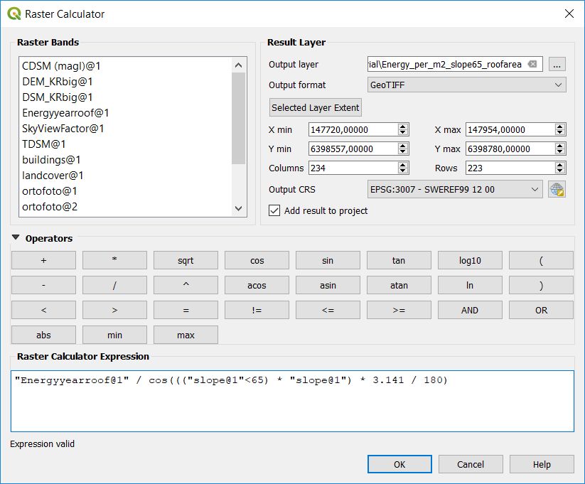
   Fig. 10 The RasterCalculator in QGIS3. Click on image for enlargement.

4. To visualize where to place solar panels, the amount of energy received needs to be cost effective. As irradiance below 900 kWh is considered to be too low for solar energy production (Per Jonsson personal communication Tyréns Consultancy), pixels lower than 900 can be filtered out (Figure below). Changing transparency allows you to make only points above a threshold of interest visible.

   • Right-click on the Energyyearroof-layer and go to Properties and then Transparency.

   • Add a custom transparency (green cross) where values between 0 and 900 are set to 100% transparency.

Irradiance map with values less than 900 kWh filtered out

To estimate solar potential on building roofs we can use the Zonal statistics tool:

1. Processing > Toolbox then search Zonal statistics. Be sure to avoid Raster layer zonal statistics.

   • Use the roof area raster layer (energy_per_m2_slope65_roofarea) created before and use building.shp as the polygon layer to calculate as your zone layer.

2. On your building layer – Right click Open Attribute Table

3. Or use identify features to click a building (polygon) of interest to see the statistics you have just calculated

   Note that we will not consider the performance of the solar panels.

   

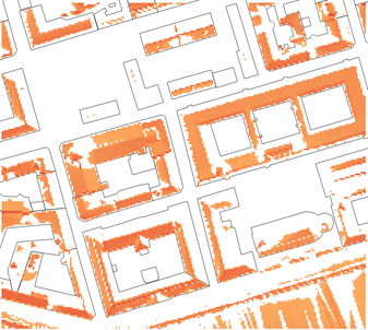
   Fig. 11 Irradiance map on building roofs in Gothenburg

Covent Garden data set

A second GIS data set is available for the Covent Garden area in London

1. Close the Gothenburg data (it may be easiest to completely close QGIS and re-open).

2. Download from the link given in the beginning of this tutorial.

3. Extract the data to a directory.

4. Load the Raster data files (as you did before).

5. Additional analysis: Shadows

   • UMEP > Processor > Solar Radiation > Daily Shadow pattern

   • Allows you to calculate the shadows for a particular time of day and Day of Year.

Questions for you to explore with UMEP:SEBE

1. Use the Gothenburg dataset consider the impact of vegetation.

   • What are the main differences between the two model runs with respect to ground and roof surfaces?

   • To what extent are the building roofs affected by vegetation?

2. Consider the differences between London and Gothenburg. You can run the model for different times of the year by modifying the meteorological data so the file only has the period of interest.

3. For Covent Garden, determine the solar energy potential for a specific building within the model domain. Work in groups to consider different areas. What would be the impact of having a smaller/larger area domain modelled for this building? Identify the possibilities of solar energy production for that building.

References

• Goodwin NR, Coops NC, Tooke TR, Christen A, Voogt JA 2009: Characterizing urban surface cover and structure with airborne lidar technology. Can J Remote Sens 35:297–309

• Lindberg F, Jonsson P, Honjo T, Wästberg D 2015: Solar energy on building envelopes - 3D modelling in a 2D environment. Solar Energy. 115, 369–378

• Ratti CF, Richens P 1999: Urban texture analysis with image processing techniques Proc CAADFutures99, Atlanta, GA

Authors of this document: Lindberg and Grimmond (2015, 2016)

Contributors to the material covered

• University of Gothenburg: Fredrik Lindberg

• University of Reading: Sue Grimmond

• Background work also comes from: UK (Ratti & Richens 1999), Sweden (Lindberg et al. 2015), Canada (Goodwin et al. 2009)

In the repository of UMEP you can find the code and report bugs and other suggestions on future improvments.

Tips

Meteorological file in UMEP has a special format. If you have data in another format there is a UMEP plugin that can convert your meteorological data into the UMEP format.

• Plugin is found at UMEP > Pre-Processor > Meteorological data >Prepare Existing data.

Plugin to visualize horisontal distributed data in 3D: called Qgis2Threejs.

• Available for download from the official repository Plugins > Manage and Install Plugins.

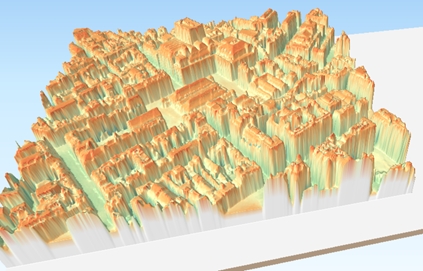
Fig. 12 3D visualisation with Qgis2Threejs over Convent Garden

TIFF (TIF) and ASC are raster data file formats. In the left Hand Side there is a list of layers.

• The layer that is checked at the top of the list is the layer that is seen, If you want to see another layer you can either:

  1. Un-tick the layers above the one you are interested in and/or

  2. Move the layer you are interested in to the top of the list by dragging it.

You can save all of you work for different areas as a project – so you can return to it as whole.

• Project > Save as…

You can change the shading etc. on different layers.

• Right Click on the Layer name Properties > Style > Singlebandpseudo color

• Choose the color band you would like.

• Classify

• Numerous things can be modified from this point.

UMEP repository.

Tutorial finished.