A First QGIS and UMEP activity
Introduction
In this exercise you will be introduced to QGIS and UMEP and some of its capabilities. You will apply a shadow casting model in Gothenburg, Sweden to investigate daliy shading patterns for pedestrians and how solar access varies with seasons and through vegetation.
Initial Practical steps
If QGIS and UMEP is not on your computer you will need to install.
When installed, UMEP can be found in the menu bar in QGIS.
Data for this Tutorial
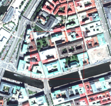
Fig. 1 Central Gothenburg study area (red square).
Geodata covers a small area in central Gothenburg, Sweden. Data are projected in SWEREF99 1200 (EPSG:3007) which is in the Swedish national coordinate system.
Datasets for Gothenburg, Sweden
You will make use of two raster datasets:
Name |
Definition |
Description |
DSM_KRbig.tif |
Ground and building DSM |
Raster dataset: derived from a 3D vector roof structure dataset and a digital elevation model (DEM) |
CDSM_KRbig.asc |
Vegetation canopy DSM |
Raster dataset: drived from a LiDAR dataset |
Add data to your QGIS project
Start by downloading the data from the link above. The data is zipped - unzip the data.
First, add DSM_KRbig.tif to your project. Use Layer > Add Layer > Add Raster Layer to open the raster file.
Examine the DSM. Your project is now using EPSG:3007 as coordinate system (CRS). This can be seen in the lower right hand side in your QGIS window.
Now add CDSM_KRbig.asc to your project. Data can also be added by drag and drop between the Browser-panel and the Layers-panel to the left.
Now you should see two layer in your Layers-panel. You should also see that CDSM_KRbig has a question mark (?) next to it. This is because no CRS is connected to this raster data. You will need to indicate the CRS that is associated with this data.
Right-click on CDSM_KRbig and go to Layer CRS -> Set Layer CRS…. Choose EPSG:3007.
When loading a dataset into QGIS, a default apperance is used. The CDSM which includes higher vegetation (trees and bushes) has the default value of zero (black) where no vegetation is present. Lets now change the apperance of the CDSM:
Right-click on CDSM_KRbig and choose Properties….
Go to the Symbology-tab and choose Singleband pseudocolor as Rendertype. Choose Greens as Color ramp. Click Apply.
Go to the Transparency-tab and add an Additional no data value of 0. Click OK.
Now you see the DSM where the CDSM has the value zero.
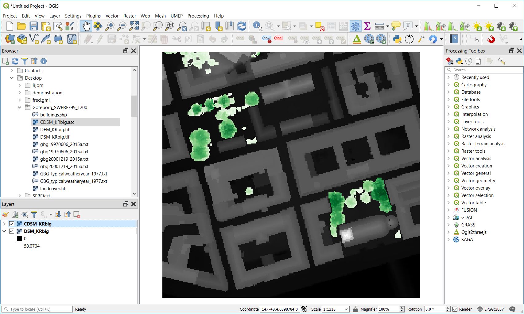
Fig. 2 The CDSM and DSM used in this exercise.
Calculate daily shadow patterns
Open the Daily Shadow Pattern tool located at UMEP -> Processor -> Solar radiation -> Daily Shadow Pattern in the menu bar.
This tool can do what its name suggests, namely calculate ground shadow patterns based on a DSM and a CDSM.
Create a directory e.g. on your Desktop called DailyShading. Also create a sub-directory to DailyShading called June21_buildings.
Use this directory to save the result.
Set-up the tool as shown in the figure below. This will generate ground shadows from buildings every 30 minutes on June 21, 2020. Click Run.
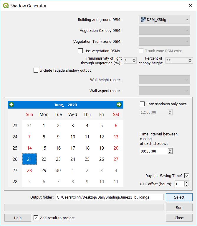
Fig. 3 Settings for calculating ground shadows from buildings with 30 minute interval on June 21, 2020.
When calculations have finished, a new layer will appear in your QGIS project (shadow_fraction_on_20200621). This layer shows the fraction (0 to 1) of sunshine for all pixels in the raster. This layer is presented with a transparancy (Global Opacity) of 50%. You can change that under the Transparency-tab for the layer.
Change the Global Opacity to 100% for easier comparison later on.
Rename shadow_fraction_on_20200621 to shadow_fraction_on_20200621_buildings by right-clicking on the layer in the Layers-panel and choose Rename Layer.
Go to the directory that you used as output folder. Here you find each individual shadow map for every 30 minute on June 21.
Now re-run with the same settings but include the CDSM as shown below. Create a new sub-directory called June21_buildingsvegetation and use this as your output location.
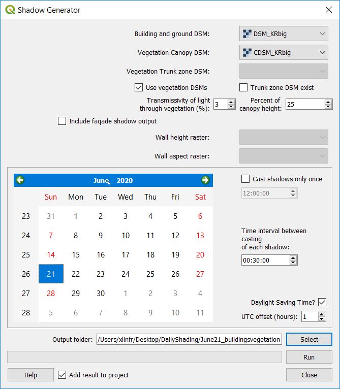
Fig. 4 Settings for calculating ground shadows from buildings and vegetation with 30 minute interval on June 21, 2020.
Rename your new shadow_fraction_on_20200621-layer to shadow_fraction_on_20200621_buildingsvegetation.
Change the Global Opacity to 100%.
Now you can compare the two created layers by tick them on and off in the Layers-panel. You can clearly see the shadows created underneath the trees.
Finally calulate shadows for December 21, 2020 using both buildings and vegetation. Now set Transparacy of light through vegeation to 50% (defoliated trees) and save the results in a sub-directory called Dec21_buildingsvegetation.
Examine the difference in shadows between the Winter and Summer solstice in Sweden Gothenburg.
Some short remarks on what you have done so far:
The building and ground DSM is critical for the calculations of shadows.
Optionally vegetation (trees and bushes) can be included as it can shadow buildings, walls and roofs, reducing the potential solar energy production.
Two vegetation DSMs are required when the Use vegetation DSMs is ticked:
One to describe the top of the vegetation (Vegetation Canopy DSM).
One to describe the bottom, underneath the canopies (Vegetation Trunk Zone DSM). As Trunk Zone DSMs are very rare, an option to create this from the canopy DSM is available.
You can set the amount of light (shortwave radiation) that is transmitted through the vegetation.
The UTC offset is needed to accurately estimate the sun position, positive numbers for easterly position and negative for westerly. For example, Gothenburg is located in CET which is UTC +1.
Use a post-processing tool to animate shadows
The UMEP plugin consists of three parts; a pre-processor, a processor and a post-processor. The pre-processor prepares spatial and meteorological data as inputs to the modelling system. The processor includes all the main models for the main calculations. To provide initial “quick looks” the post-processor will enable results to be plotted, statistics calculated etc. Based on the model output. Now you will use a post-processing plugin to examine the shadow pattern you have generated in this tutorial more closely.
Go to UMEP -> Post-Processor -> Outdoor Thermal Comfort -> SOLWEIG Analyzer. We will “borrow” this tool to animate the shadows we created earlier.
Load one of three output folders you have used in this exercise.
Click on Show Animation
Now you will see a short animation of the shadow patterns at 30 minute intervals for the data that you generated with the Daily Shadow Pattern-tool.
Tutorial finished.