This tutorial demonstrates how the GQF software is used to simulate
anthropogenic heat fluxes (QF) for London, UK, in the year 2015, using a
mixture of administrative and meteorological data.
UMEP is a python plugin used in conjunction with
QGIS. To install the software and the UMEP
plugin see the getting
started
section in the UMEP manual.
As UMEP is under constant development, some documentation may be missing
and/or there may be instability. Please report any issues or suggestions
to our repository.
GQF uses multiple shapefiles (ending .shp) to build up a picture of
energy use, population and road transport across the city. Five pieces
of information are needed for each of these:
Filename: The full path to the .shp file (e.g.
c:\path\to\file.shp)
Start date: The modelled date from which this data should be used
EPSG code: A numeric code that determines which co-ordinate reference
system (CRS) to use for the shapefile
Attribute to use. A shapefile attaches one or more attributes (e.g.
population or energy consumption) to each spatial unit. The name of
the relevant attribute must be specified here.
Feature IDs: The name of an attribute that contains a unique
identifier for each spatial unit
Click here
for a guide explaining how to identify the feature ID, attribute to use
and EPSG code of a shapefile using QGIS.
A shapefile also defines the so-called output areas, which are the
spatial units (sometimes pixels) of model output (one QF estimate per
area). These are needed because the spatial units of the various input
files may not all match up. The output areas can either be one of the
input files, or a totally different set of areas. In this tutorial, one
of the population datasets is used to keep things simple.
The data sources file needs to be updated so that it can find the
various data files, and understands what to do with them. A full
description of the Data sources file contents is available
here, but this section shows how to
build up the entries.
There are several sections in the data sources file. Each is bounded by
§ion_name and ends with “/” and deals with a different part
of the input data.
Open DataSources.nml using a text editor (we recommend Notepad++).
The following steps show how to update the entries according to the
information gathered above.
The epsgCode and featureIds entries are found by inspecting
each file using QGIS. Note that each file has different values for
these
The attribToUse entry for each file is covered in the table above
An arbitrary start date of 2011-01-01 (1st january) can be used for
the data shown.
For brevity, just the first two sections of the DataSources.nml file are
shown here: Using the workday population spatial units as model output
areas. This section does not need to use an attribute or know about a
start date:
! ### Population data
&residentialPop
   shapefiles = 'C:\path\to\data\500m_Residential_from_100m.shp'
   startDates = '2011-01-01'
   attribToUse = 'Pop'
   featureIds = 'ID'
/
The same pattern is used for the other spatial input datasets:
workplacePop: Workplace/workday population dataset
annualIndGas: Industrial gas use
annualIndElec: Industrial electricity use
annualDomGas: Domestic gas use
annualDomElec: Domestic electricity use (same file as domestic
gas, but different attribute)
For the annualEco7 section, we shall assume zero consumption. This
doesn’t need a shapefile - a single number indicating the whole-city
consumption should be used instead, along with dummy EPSG code,
attribToUse and featureIds:
&annualEco7
   ! Spatial variations of economy 7 electricity use
   shapefiles = 0.0
   startDates = '2014-01-01'
   epsgCodes = 1
   attribToUse = 'IndGas' !A dummy name
   featureIds = ''
/
GQF uses annual total energy consumption shapefiles, and needs to know
how to vary energy consumption on different dates (e.g. winter is likely
to have more fuel use than summer). This is captured using real data
from the energy grid. The 2015GasElecDD.csv file contains each day’s
total gas and electricity consumption. GQF then scales the annual
consumption based on this each day.
Only the year(s) represented by the data should be modelled, but if only
past years are available GQF will recycle it for later years, offering
the closest sensible match to time of week and time of year.
How much energy each the average person emits at each time of day
The fraction of an area’s workday population actually at work (and by
extension the fraction of the residential population at home)
The metabolism.csv file contains a weekday, saturday and sunday
variant of this information, and copies for each daylight savings regime
in the UK to account for changes in the summer.
! Temporal metabolism data
&diurnalMetabolism
    profileFiles = 'N:\QF_London\GreaterQF_input\London\Profiles\\Metabolism.csv'
/
As shown above, the different kinds of building energy consumption are
separated in GQF. Their diurnal profiles are also different so that the
different behaviours of households and businesses are represented
accurately. This means that each of the building energy inputs also
requires a diurnal profile data file:
&diurnalDomElec
   ! Diurnal variations in total domestic electricity use (metadata provided in file; files can contain multiple seasons)
   profileFiles =
'C:\Path\To\BuildingLoadings_DomUnre.csv'
/
&diurnalDomGas
   ! Diurnal variations in total domestic gas use (metadata provided in file; files can contain multiple seasons)
   profileFiles = 'C:\Path\To\BuildingLoadings_DomUnre.csv'
/
&diurnalIndElec
   ! Diurnal variations in total industrial electricity use (metadata provided in file; files can contain multiple seasons)
   profileFiles = 'C:\Path\To\BuildingLoadings_Industrial.csv'
/
&diurnalIndGas
   ! Diurnal variations in total industrial gas use (metadata provided in file; files can contain multiple seasons)
   profileFiles = 'C:\Path\To\BuildingLoadings_Industrial.csv'
/
&diurnalEco7
   ! Diurnal variations in total economy 7 electricity use (metadata provided in file; files can contain multiple seasons)
   profileFiles = 'C:\Path\To\BuildingLoadings_EC7.csv'
/
To save time, the DataSources file is mostly completed in advance with
entries that reflect the transport shapefile, but some of the key
entries still need completing as part of the tutorial:
The location, EPSG code, feature ID and start date of the road
transport shapefile
Information about what is available in the shapefile
It should be possible to complete and/or verify the first four entries
using the table and information above.
The next three entries should be all be set to 1 to signify that they
are provided by the shapefile
speed_available: vehicle speed provided for each road link
total_AADT_available: annual average daily traffic (traffic flow)
provided for each road link
vehicle_AADT available: AADT is broken down by vehicle type for each
road link
&transportData
  ! Vector data containing all road segments for study area
  shapefiles = 'C:\path\to\data\LAEI2013_AADTVKm_2013_link.shp'
  startDates = '2008-01-01'
  epsgCodes = 27700
  featureIds = 'OBJECTID'
  ! What data is available for each road segment in this shapefile? 1 = Yes; 0 = No
  speed_available = 1                 ! Speed data. If not available then default values from parameters file are used
  total_AADT_available = 1            ! Total annual average daily total (AADT: total vehicles passing over each segment each day)
  vehicle_AADT_available = 1          ! AADT available for specific vehicle types
/
The rest of the section tells GQF which attributes to use for various
aspects of the traffic data, and what different kinds of roads are
called:
    ! Road classification information. This is used with assumed values for AADT
    class_field = 'DESC_TERM'           ! The shapefile attribute that contains road classification
    ! Strings that identify each class of road
    motorway_class = 'Motorway'
    primary_class = 'A Road'
    secondary_class = 'B Road'
    ! All other road types will be considered as \ “other”
    ! Average speed for each road segment
    speed_field = 'Speed_kph'           ! Field name
    speed_multiplier = 1.0              ! Factor that converts data to km/h (1.0 if data is already in km/h)
    ! Annual average daily total (mean number of vehicles per day) passing over each road segment in the shapefile
    ! Specify attribute names if data is present in the shapefile.
    AADT_total = 'AADTTOTAL'            ! Total AADT for all vehicles. Leave blank ('') if not available
    ! AADT for cars of different fuels (leave as '' if not available)
    AADT_diesel_car = 'AADTDcar'        ! Petrol cars
    AADT_petrol_car = 'AADTPcar'        ! Diesel cars
    ! Secondary option: Use total AADT for cars and break down using assumed fuel fractions from model parameters file
    AADT_total_car = ''               ! Total AADT for all cars (required if the other car fields are ''; ignored if they are specified)
    ! AADT for LGVs of different fuels leave as '' if not available)
    AADT_diesel_LGV = 'AADTDLgv'        ! Petrol LGVs
    AADT_petrol_LGV = 'AADTPLgv'        ! Diesel LGVs
    ! Secondary option: Use total LGV AADT and assumed fuel fractions from parameters file
    AADT_total_LGV = ''               ! Total AADT for all LGVs (required if the other LGV fields are ''; ignored if they are specified)
    ! AADT for other vehicles. These are broken down into diesel/petrol based on fuel fractions (see model parameters file)
    ! Specify shapefile attribute name or leave as '' if not available
    AADT_motorcycle = 'AADTMotorc'      ! Motorcycles
    AADT_taxi = 'AADTTaxi'              ! Taxis
    AADT_bus = 'AADTLtBus'                  ! Buses
    AADT_coach = 'AADTCoach'                ! Coaches
    AADT_rigid = 'AADTRigid'                ! Rigid goods vehicles
    AADT_artic = 'AADTArtic'                ! Articulated trucks
/
The fuelConsumption.csv file contains a list of vehicle fuel efficiency
by fuel, vehicle type and era. This is used to calculate each road
link’s fuel consumption:
&fuelConsumption
   ! File containing fuel consumption performance data for each vehicle type as standards change over the years
   profileFiles = 'C:\Path\To\fuelConsumption.csv'
/
Each vehicle type has a different activity profile. For example, freight
and taxi vehicle may operate later at night than passenger cars. The
Transport.csv file contains a profile for each of these:
&diurnalTraffic
   ! Diurnal cycles of transport flow for different vehicle types
   profileFiles = 'C:\Path\To\Transport.csv'
/
Each profile is a week long, and these profiles control changes to the
total volume of traffic each day.
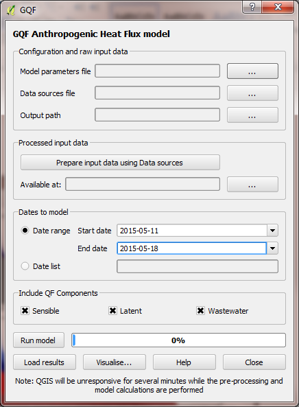
Working from the top of the dialog box to the bottom…
Click the … buttons in the Configuration and raw input data panel
to browse to the parameters.nml and DataSources.nml files. A pop-up
error message will warn of any problems inside the files.
Output path: A folder in which the model outputs will be stored.
It is strongly recommended that a new folder is used each time.
Click Prepare input data using Data Sources button. This may be a
time-consuming step: It matches the various inputs to each output
area. Where output areas and input shapes are not identical, it also
splits population or energy use across output areas based on their
overlapping fractions.
Once this step is complete, the available at: box will become
populated. This folder contains the disaggregated data needed to run
the model.
Tip: Save time in future: If the exact same input data files are
used in a later study, then the “prepare” step can be skipped: click the
“…” button and navigate to a folder that contains the relevant
disaggregated data. It will then be copied to the new output folder and
used as normal.
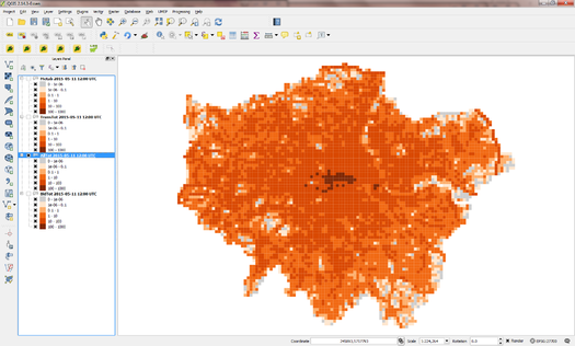
Use the visualisation tool to create a map of all the QF components at
noon (11:00-12:00 UTC) on May 11 by selecting that time and pressing
Add to canvas. This may take a moment to process. Close the
visualisation took and return to the main canvas to inspect the four new
layers that have appeared.
Each layer corresponds to a different QF component:
Metab: Metabolism
TransTot: Total from all road transport sources
AllTot: Total QF from all emissions
BldTot: Total building emissions
De-selecting a layer in the Layers panel removes it from view.
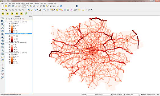
Leaving just AllTot (total QF ) visible, there isn’t much structure in the
colours.
Add some contrast to it by choosing a different colour scale:
Right-click the QF layer, go to Properties > Style, change the colour
ramp to “Reds” and choose Mode: Natural Breaks (Jenks). This shows much
more structure, although the grid borders are distracting. These can be
removed by double-clicking the colour levels and choosing a border
colour the same as the fill colour.
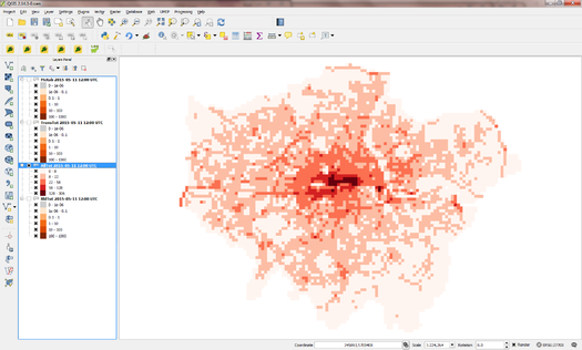
The roads have a very different spatial pattern to buildings, so these
can also be visualised by selecting the TransTot layer and re-colouring
accordingly:
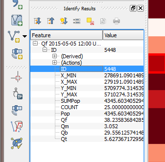
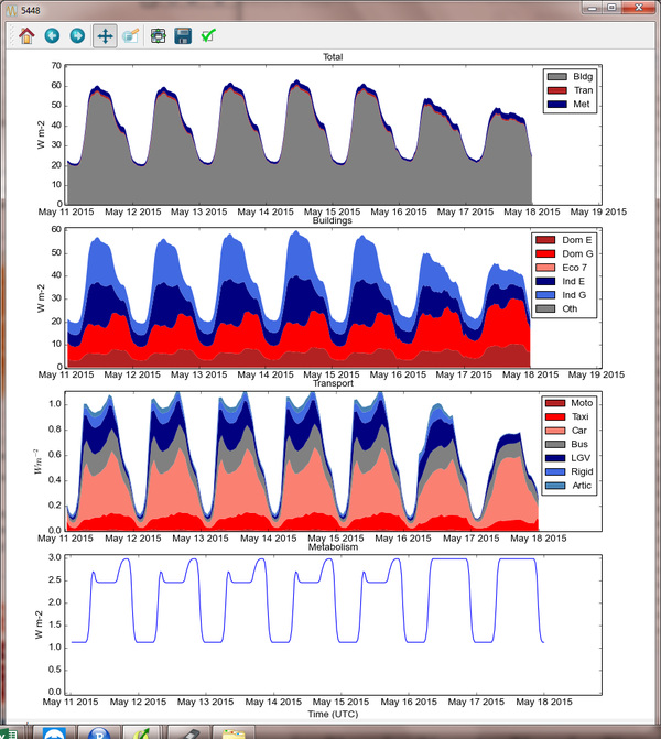
Return to the visualisation tool, choose output area 5448 and click
show plot. Time series of each QF component then appear for the week.
Note the lower traffic activity and different behaviours on Saturday and
Sunday, when people are expected to not be at work.
The parameters.nml file contains three entries related to public
holidays, which are treated as the second day of the weekend by GQF:
Use_UK_holidays: Religious and recurrent public holidays from the
UK are calculated automatically
Use_custom_holidays: Set to 1 in order to have GQF read in a list
of user-provided holidays
custom_holidays: A comma-separated list of dates that should be
treated as holidays in format YYYY-mm-dd (e.g. “2015-05-07”,
“2015-07-30”)
In this example, a fictional public holiday of 2015-05-13 is entered
into the parameters.nml file. The model is then run as in Tutorial 1,
and the resulting time series in output area 5448 is shown below:
Fig. 74 Time series with extra public holiday on May 13
Compared against the results from Tutorial 1, the curve on May 13 in
each sub-plot now resembles May 17 (a Sunday) rather than the weekdays
around it.
Sensible: Transported by convection (usually the largest share)
Latent: Transported by the vaporisation of water
Wastewater: Heat in water ejected by buildings
GQF includes all of these in the calculated fluxes by default, but one
or more of them can be removed at model run-time using the checkboxes:
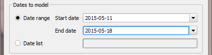
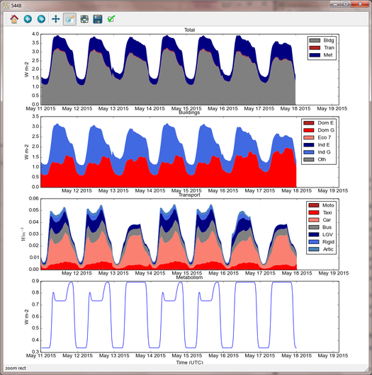
In this example, the week of 11 to 18 May 2015 is again modelled but the
“Sensible” and “Wastewater” checkboxes are un-ticked. This means the
modelled QF will contain only latent heat. The resulting time series in
area 5448 is shown below:
Fig. 75 Time series with only latent and wastewater contributions included, and extra public holiday on May 13
The emissions are far lower than those in Tutorial 2a, showing how
latent heat is a relatively small contribution. Consuming electricity
emits no latent heat, unlike gas, while metabolism now represents a
larger fraction of the total.